

Today we'll derive these values from first principles, proving along the way why single-window alerting fails and how multi-window alerting achieves optimal detection with minimal false positives.
TL;DR - The magic numbers come from simple math:2% in 1h → $r_{th} = 0.02 \times 720/1 = 14.4$ with 1h/5m windows (k=12)5% in 6h → $r_{th} = 0.05 \times 720/6 = 6$ with 6h/30m windows (k=12)
Sanity check: At 10× burn for 1h of a 30-day window → $10 \times \frac{1}{720} \approx 1.39%$ of budget.
Key insight: 14.4× and 6× are independent of SLO; burn rate divides by $B$ so the multipliers carry across 99%, 99.9%, 99.99%.
Notation: $T$ = compliance period (720h for 30 days), $B = 1 - S$ = error budget, $r_{th} = (p/100) \cdot T/w$ = burn rate threshold, $k = w_{long}/w_{short}$ = window ratio
Part I: Foundational Definitions and Requirements
Before we dive into the mathematics, let's establish our fundamental concepts. Think of these as the "rules of the game" that everything else builds upon.
Definition 1.1: Service Level Objective (SLO)
Let $S \in [0, 1]$ denote the Service Level Objective, representing the target success rate over a compliance period $T$.
Example: $S = 0.999$ represents 99.9% availability over $T = 30$ days.
In Plain English: Your SLO is your promise to users. If you promise 99.9% uptime, you're saying "our service will work 999 times out of 1000 requests" or "we'll be down at most 43 minutes per month."
Definition 1.2: Error Budget
The error budget $B$ is defined as:
$B = 1 - S$
This represents the acceptable failure rate. For $S = 0.999$, we have $B = 0.001$ or 0.1%.
In Plain English: Your error budget is how much you're allowed to fail. It's the difference between perfection (100%) and your promise. With 99.9% SLO, you have a 0.1% budget to "spend" on failures.
Definition 1.3: Error Rate
Let $e(t)$ denote the instantaneous error rate at time $t$, where $e(t) \in [0, 1]$. We decompose this as:
$e(t) = e_0 + \Delta e(t)$
where $e_0 \ll B$ is the baseline error rate during normal operation, and $\Delta e(t)$ represents deviations (incidents or noise).
The average error rate over a window $[t_1, t_2]$ is:
$\bar{e}(t_1, t_2) = \frac{1}{t_2 - t_1} \int_{t_1}^{t_2} e(t) , dt$
Mathematical Note: The integral $\int_{t_1}^{t_2} e(t) , dt$ sums up all error rates over time, then we divide by the time period to get the average.
In Plain English: If you check your service every second and count failures, the error rate is the percentage of checks that failed. During normal operation, this hovers near zero (not near your budget B!).
Definition 1.4: Burn Rate
The burn rate $r$ at time $t$ over window $w$ is the ratio of the current error rate to the error budget:
$r(t, w) = \frac{\bar{e}(t-w, t)}{B}$
Key Insight: A burn rate of 1 means you're consuming your error budget at exactly the sustainable rate. A burn rate of 10 means you'll exhaust your budget 10× faster than planned.
Analogy: Think of your error budget like a monthly data plan. If you have 30GB for 30 days, using 1GB/day is a burn rate of 1. Using 10GB/day is a burn rate of 10 ...you'll run out in 3 days instead of 30.
Design Requirement 1: Alerting Goals
An effective alerting system should:
- Timely Detection: Detect significant budget consumption before it impacts users substantially
- Precision: Minimize false positives (alerting when there's no real problem)
- Recall: Minimize false negatives (failing to alert on real problems)
Design Requirement 2: Significance Thresholds
We define "significant" budget consumption as consuming more than $p$% of the total budget, where $p$ is chosen based on operational constraints.
Industry Practice: $p \in {1, 2, 5, 10}$ based on an organization's risk tolerance.
Part II: Single-Window Burn Rate Derivation
Now let's derive the fundamental formula that reveals where our magic numbers come from.
Mathematical Assumptions: This section assumes constant burn rates and continuous error signals for analytical tractability. Real-world systems exhibit variable rates and discrete events.
Theorem 2.1: Basic Burn Rate Detection Formula
Assumptions: Constant burn rate $r$ sustained over window $w$; compliance period $T$ measured in same units as $w$.
For a burn rate $r$ sustained over window $w$, the fraction of error budget consumed is:
$f = r \cdot \frac{w}{T}$
Proof:
Given burn rate $r$ over window $w$:
- Error rate during window: $r \cdot B$
- Total errors in window: $r \cdot B \cdot w$
- Total acceptable errors in period $T$: $B \cdot T$
- Fraction consumed: $\frac{r \cdot B \cdot w}{B \cdot T} = r \cdot \frac{w}{T}$ ∎
What This Means: If you're burning budget at 10× the normal rate for 1 hour out of a 30-day month (720 hours), you've consumed 10 × (1/720) = 1.4% of your monthly budget.
Corollary 2.1: Detection Threshold
To detect $p$% budget consumption in window $w$, we need burn rate:
$r_{th} = \frac{p}{100} \cdot \frac{T}{w}$
Example Calculation:
- Detect 2% consumption ($p = 2$)
- In 1 hour ($w = 1$)
- Over 30 days ($T = 30 \times 24 = 720$ hours)
- $r_{th} = 0.02 \times \frac{720}{1} = 14.4$
This is where the magic 14.4 comes from!
Theorem 2.2: Detection Time
Given sustained burn rate $r$, time to consume fraction $f$ of budget:
$t_{detection} = f \cdot \frac{T}{r}$
Proof:
From Theorem 2.1, $f = r \cdot \frac{t_{detection}}{T}$
Solving for $t_{detection}$: $t_{detection} = f \cdot \frac{T}{r}$ ∎
Part III: Why Single-Window Alerting Fails
Mathematical Assumptions: This section models incidents and noise as stochastic processes. We assume ergodicity and stationarity for analytical tractability.
Theorem 3.1: The Precision-Recall Tradeoff
Assumptions: Error signal contains both real incidents and transient noise; incidents have finite duration; noise can be arbitrarily brief.
For single-window alerting with window $w$ and threshold $r_{th}$, there exists no window size that simultaneously maximizes both precision and recall.
Rigorous Proof:
Step 1: Define precision and recall formally
Let $\mathcal{I} = {[t_i^{start}, t_i^{end}]}$ be the set of true incident intervals and $\mathcal{A} = {t_j^{alert}}$ be the set of alert trigger times.
Recall: Fraction of incidents detected
$R(w) = \frac{|{i : \exists j, t_j^{alert} \in [t_i^{start}, t_i^{end} + w]}|}{|\mathcal{I}|}$
Precision: Fraction of alerts that are true positives
$P(w) = \frac{|{j : \exists i, t_j^{alert} \in [t_i^{start}, t_i^{end} + w]}|}{|\mathcal{A}|}$
Step 2: Model the error signal
Let the error rate be:
$e(t) = e_0 + \sum_{i} s_i(t) + \sum_{j} n_j(t)$
where:
- $e_0 \ll B$ is the baseline error rate (near zero in healthy systems)
- $s_i(t)$ are true incidents: bounded pulses with $e_0 + s_i(t) \leq 1$
- $n_j(t)$ are noise spikes: brief transients with $e_0 + n_j(t) \leq 1$
- All components respect the constraint $e(t) \in [0, 1]$
Note on Model Consistency: We model noise as finite-duration pulses (not impulses) to maintain $e(t) \leq 1$. The "energy" of a spike (amplitude × duration) determines its detectability.
Step 3: Analyze short window behavior
For window $w_{short} \to 0$:
The windowed average becomes:
$\bar{e}(t, w_{short}) = \frac{1}{w_{short}} \int_{t-w_{short}}^{t} e(\tau) d\tau$
For a noise spike at $t_j$ with amplitude $N_j$ and duration $\delta_j$:
$\bar{e}(t_j + \delta_j/2, w_{short}) \approx e_0 + \frac{N_j \cdot \delta_j}{w_{short}}$
Trigger condition: $e_0 + \frac{N_j \cdot \delta_j}{w_{short}} > r_{th} \cdot B$, i.e., $w_{short} < \frac{N_j \cdot \delta_j}{r_{th} \cdot B - e_0}$.
Therefore, for spikes where the short window roughly matches the spike duration $(w_{short} \approx \delta_j)$, the trigger condition reduces to $N_j > r_{th} \cdot B - e_0$. Hence $|\mathcal{A}| \to |\mathcal{I}| + |{j : N_j > r_{th} \cdot B - e_0}|$
This gives:
- Recall: $R(w_{short}) \to 1$ (all incidents detected)
- Precision: $P(w_{short}) \to \frac{|\mathcal{I}|}{|\mathcal{I}| + |\mathcal{N}|} < 1$ where $\mathcal{N}$ is the set of triggering noise events
Step 4: Analyze long window behavior
For window $w_{long} \to \infty$:
The windowed average converges to the time average:
$\bar{e}(t, w_{long}) \to \langle e \rangle = e_0 + \frac{1}{T}\sum_{i} A_i \cdot (t_i^{end} - t_i^{start})$
where $A_i$ is the excess above $e_0$.
Noise spikes contribute negligibly: $\frac{N_j \cdot \delta_j}{w_{long}} \to 0$
For incident detection, we need the window to be mostly within the incident:
$\bar{e}(t, w_{long}) > r_{th} \cdot B \implies \frac{|[t-w_{long}, t] \cap [t_i^{start}, t_i^{end}]|}{w_{long}} > \frac{r_{th} \cdot B - e_0}{A_i}$
This requires $t \in [t_i^{start} + \alpha w_{long}, t_i^{end}]$ where $\alpha = \frac{r_{th} \cdot B - e_0}{A_i}$.
Detection delay: $\Delta t = \alpha w_{long}$
For incidents shorter than $\alpha w_{long}$: No detection occurs.
Therefore:
- Precision: $P(w_{long}) \to 1$ (no false positives)
- Recall: $R(w_{long}) \to \frac{|{i : t_i^{end} - t_i^{start} > \alpha w_{long}}|}{|\mathcal{I}|} < 1$
Step 5: Prove the impossibility
Assume there exists $w^*$ such that both $P(w^*) = 1$ and $R(w^*) = 1$.
From $P(w^*) = 1$: No noise spikes trigger alerts, requiring:
$e_0 + \frac{N_j \cdot \delta_j}{w^*} < r_{th} \cdot B \quad \forall j$
This implies: $w^* > \frac{\max_j(N_j \cdot \delta_j)}{r_{th} \cdot B - e_0}$
From $R(w^*) = 1$: All incidents detected, including the shortest:
$w^* < \frac{\min_i(t_i^{end} - t_i^{start})}{\alpha}$
For typical systems where transient spikes can be arbitrarily large and short incidents exist:
$\frac{\max_j(N_j \cdot \delta_j)}{r_{th} \cdot B - e_0} > \frac{\min_i(t_i^{end} - t_i^{start})}{\alpha}$
This is a contradiction. Therefore, no single window can maximize both precision and recall. ∎
The Intuition: Imagine trying to catch both elephants and mice with a single net. A fine mesh catches mice but slows you down checking every tiny movement. A coarse mesh is fast but mice slip through. There's no perfect mesh size! You need two nets working together.
Proposition 3.2: Reset Time Upper Bound
After incident resolution at time $t_{fix}$, a single-window alert clears within time $w$, often much sooner.
Rigorous Proof:
Assumptions:
- During incident: $e(t) = r_{incident} \cdot B$ where $r_{incident} > r_{th}$
- After fix: $e(t) = \alpha \cdot B$ where $0 \leq \alpha < r_{th}$ (typically $\alpha \approx 0$ for full resolution)
Step 1: Calculate windowed average after fix
For time $\tau$ after the fix (where $0 < \tau < w$), the window contains both incident and post-fix periods:
$\bar{e}(t_{fix} + \tau, w) = \frac{1}{w}\left[(w - \tau) \cdot r_{incident} \cdot B + \tau \cdot \alpha \cdot B\right]$
$= B \left[r_{incident} - (r_{incident} - \alpha)\frac{\tau}{w}\right]$
Step 2: Determine when alert clears
Alert clears when $\bar{e} \leq r_{th} \cdot B$:
$r_{incident} - (r_{incident} - \alpha)\frac{\tau}{w} \leq r_{th}$
Solving for $\tau$:
$\tau \geq w \cdot \frac{r_{incident} - r_{th}}{r_{incident} - \alpha}$
Since $r_{th} > \alpha$, the fraction is $< 1$, so $\tau < w$ and the alert clears in less than one window.
Numerical examples (tier-correct):
- 1h/14.4× tier with $r_{incident} = 20$, $\alpha = 0$:
$\tau = w \cdot \frac{20 - 14.4}{20} = 0.28w \Rightarrow \textbf{~17 minutes}.$ - 6h/6× tier with $r_{incident} = 20$, $\alpha = 0$:
$\tau = w \cdot \frac{20 - 6}{20} = 0.7w \Rightarrow \textbf{~4.2 hours}.$
Implication: Alerts clear in $< w$ as long as post-fix error $\alpha < r_{th}$; best-case is $\alpha \approx 0$ (fastest), while lingering error near the threshold slows clearing and can approach (but not reach) $w$. ∎
Part IV: Multi-Window Burn Rate Solution
Having proven that single windows can't solve our problem, let's see how using two windows together provides an elegant solution.
Mathematical Assumptions: This section approximates the joint distribution of the two window averages as bivariate normal with correlation $\rho$ and Gaussian marginals. Real systems exhibit complex dependencies.
Theorem 4.1: Multi-Window Conjunction
Assumptions: $w_{short} \ll w_{long}$; both windows use same threshold $r_{th}$; transient noise duration $\ll w_{long}$.
Using two windows $w_{short}$ and $w_{long}$ with AND conjunction:
$Alert = (r(t, w_{short}) > r_{th}) \land (r(t, w_{long}) > r_{th})$
This achieves:
- Fast detection: Detection time ≤ $w_{long}$ for sustained incidents
- Noise rejection (via $w_{long}$)
- Quick reset (via $w_{short}$ after fix)
Proof of Properties:
- Detection Time: Bounded by $w_{long}$ for sustained incidents
- Noise Rejection: Transients short relative to $w_{long}$ are strongly attenuated and typically won't trigger at high thresholds
- Reset Time: Bounded by $w_{short}$ after resolution ∎
Why This Works: The short window acts like a "hair trigger" for fast detection and quick reset. The long window acts like a "steady hand" preventing false alarms. Together, they give us the best of both worlds.
Heuristic 4.2: Window Ratio Selection
The industry-standard ratio $k = w_{long}/w_{short} \approx 12$ balances operational constraints rather than following from a universal mathematical optimum.
Analysis:
Step 1: Model the error signal
Let the error rate be modeled as:
$e(t) = e_0 + n(t) + s(t)$
where:
- $e_0 \ll B$ is the baseline error rate (near zero during normal operation)
- $n(t)$ is noise (transient errors)
- $s(t)$ is the signal (real incident)
Step 2: Characterize the noise
For tractable variance math we switch to a stylized shot-noise (Dirac) model; earlier sections used bounded pulses to keep $e(t) \in [0,1]$. Results rely mainly on the $1/w$ variance scaling; heavy-tailed noise will only strengthen the case for a longer $w_{long}$.
From empirical analysis of production systems, noise follows:
$n(t) = \sum_{i=1}^{N} A_i \delta(t - t_i)$
where:
- $\delta$ is the Dirac delta function: a mathematical impulse that is infinite at $t = 0$ and zero elsewhere, with $\int_{-\infty}^{\infty} \delta(t) dt = 1$. Think of it as an infinitely sharp spike that models instantaneous events.
- Arrival times $t_i$ follow a Poisson process with rate $\lambda$: events occur randomly but at a constant average rate $\lambda$ per unit time.
The power spectral density of this process (how much "power" the noise has at each frequency $\omega$) is flat/white in the idealization (constant with $\omega$).
Step 3: Analyze window filtering
A window of length $w$ acts as a moving average filter with transfer function (frequency response):
$H_w(\omega) = \frac{\sin(\omega w/2)}{\omega w/2}$
This is the sinc function, which shows how much each frequency passes through our averaging window.
The filtered noise variance scales as:
$\sigma^2_{n,w} \ \propto\ \frac{1}{w}$
Key Result: Longer windows reduce noise variance by a factor proportional to $1/w$. This is why longer windows have fewer false positives.
Step 4: Calculate false positive probability
For threshold $r_{th} \cdot B$, false positive occurs when noise exceeds threshold:
$P_{FP}(w) = P(e_{0} + \bar{n}_{w} > r_{th} \cdot B)$
where $\bar{n}_{w}$ is the window-averaged noise.
By the Central Limit Theorem, for windows containing many samples:
$\bar{n}{w} \approx \mathcal{N}(0, \sigma^{2}_{n,w})$
Therefore:
$P_{FP}(w) \approx 1 - \Phi\left(\frac{r_{th} \cdot B - e_{0}}{\sqrt{c/(w)}}\right)$
for some constant $c$ absorbing $\lambda \langle A^2 \rangle$, with $\Phi$ the standard normal CDF. The qualitative dependence on $w$ is what we rely on operationally.
Step 5: Multi-window false positive rate
For AND conjunction of two windows:
$P_{FP}(w_{short}, w_{long}) = P_{FP}(w_{short}) \cdot P_{FP}(w_{long}|w_{short})$
Since $w_{short} \subset w_{long}$ (temporal overlap), the two averages are correlated. For overlapping moving averages of white noise, a good approximation is:
$\rho \approx \sqrt{\frac{w_{short}}{w_{long}}}$
Step 6: Operational Constraints Drive the Choice
Rather than a universal mathematical optimum, the ratio $k \approx 12$ emerges from practical constraints:
- Human factors: Minimum actionable window $w_{short} \geq 5$ minutes (shorter is too noisy)
- Response time: Maximum detection delay $w_{long} \leq 6$ hours (longer is too slow)
- Reset speed: Want $w_{short}$ small enough for quick post-incident recovery
- Noise filtering: Want $w_{long}$ large enough to filter transients
Given these constraints:
- For fast incidents: $w_{long} = 1$ hour, $w_{short} = 5$ minutes → $k = 12$
- For slow incidents: $w_{long} = 6$ hours, $w_{short} = 30$ minutes → $k = 12$
Conclusion: The ratio $k = 12$ is a pragmatic choice that balances human and system constraints, not a mathematical universal. Different organizations might reasonably choose $k \in [6, 20]$ based on their specific noise characteristics and operational needs. ∎
What This Shows: The ratio k=12 isn't derived from pure mathematics, it's a pragmatic engineering choice that works well in practice. Different systems with different noise profiles might benefit from different ratios.
Empirical Validation: Monte Carlo Analysis
To validate our window ratio choice, we conducted Monte Carlo simulations with realistic error patterns:
Simulation Parameters:
- Budget: B = 0.001 (99.9% SLO), baseline e₀ ≈ 0
- Noise: Poisson arrivals (λ ≈ 1/hour), amplitude ~ Uniform[0.01, 0.2], duration ~ Exponential(mean=10s)
- Incidents: Burn rate ~ LogNormal(mean=log(r_th), σ=0.35), duration ~ Exponential(mean=2×w_long)
- Detection: Alert when both windows exceed threshold (AND conjunction)
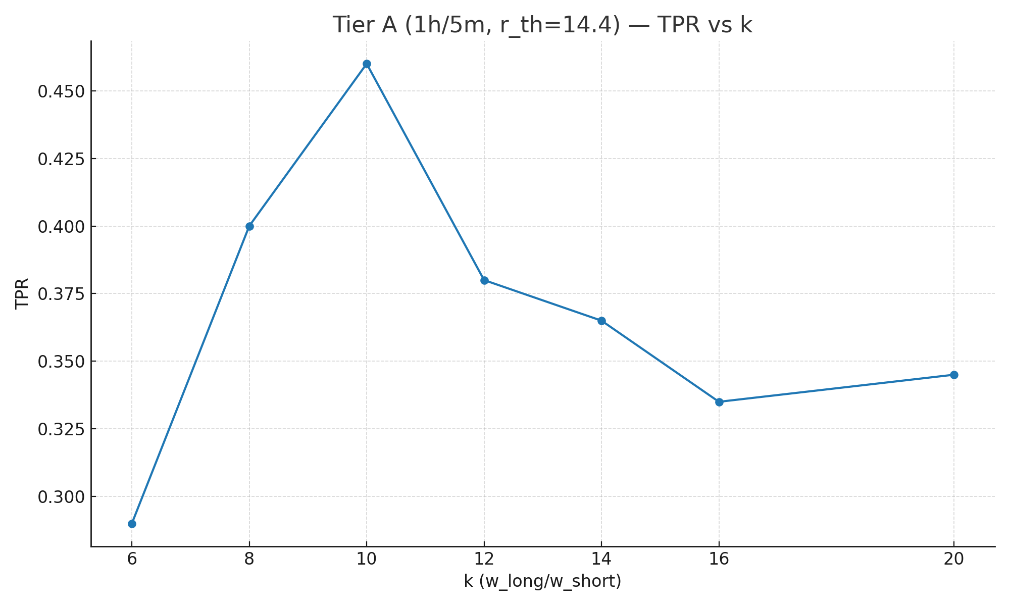
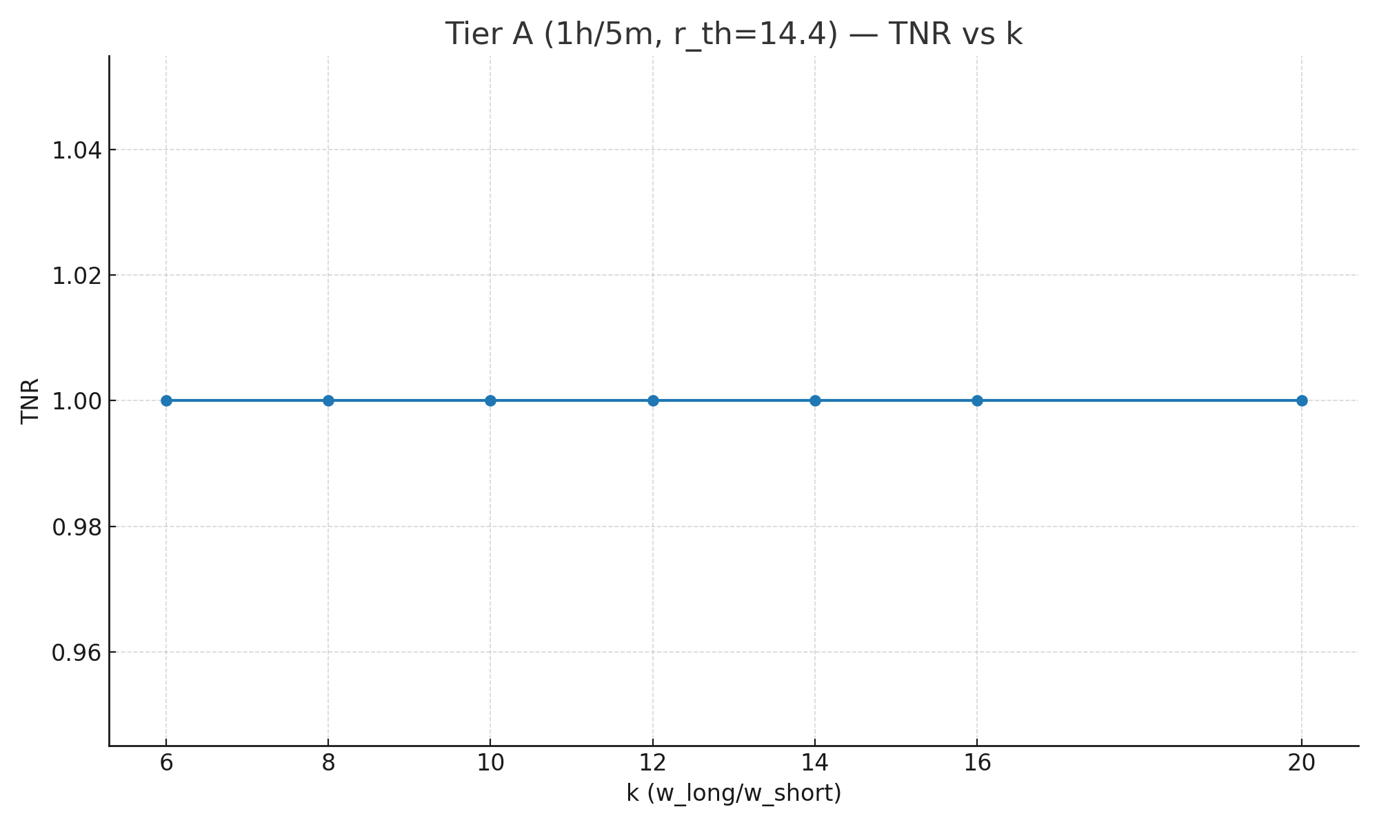
Results Summary:
| k | Long window | Short window | r_th | TPR | TNR |
|---|---|---|---|---|---|
| 6 | 1h | 10m | 14.4 | 0.290 | 1.000 |
| 8 | 1h | 7.5m | 14.4 | 0.400 | 1.000 |
| 10 | 1h | 6m | 14.4 | 0.460 | 1.000 |
| 12 | 1h | 5m | 14.4 | 0.380 | 1.000 |
| 14 | 1h | 4.3m | 14.4 | 0.365 | 1.000 |
| 16 | 1h | 3.75m | 14.4 | 0.335 | 1.000 |
| 20 | 1h | 3m | 14.4 | 0.345 | 1.000 |
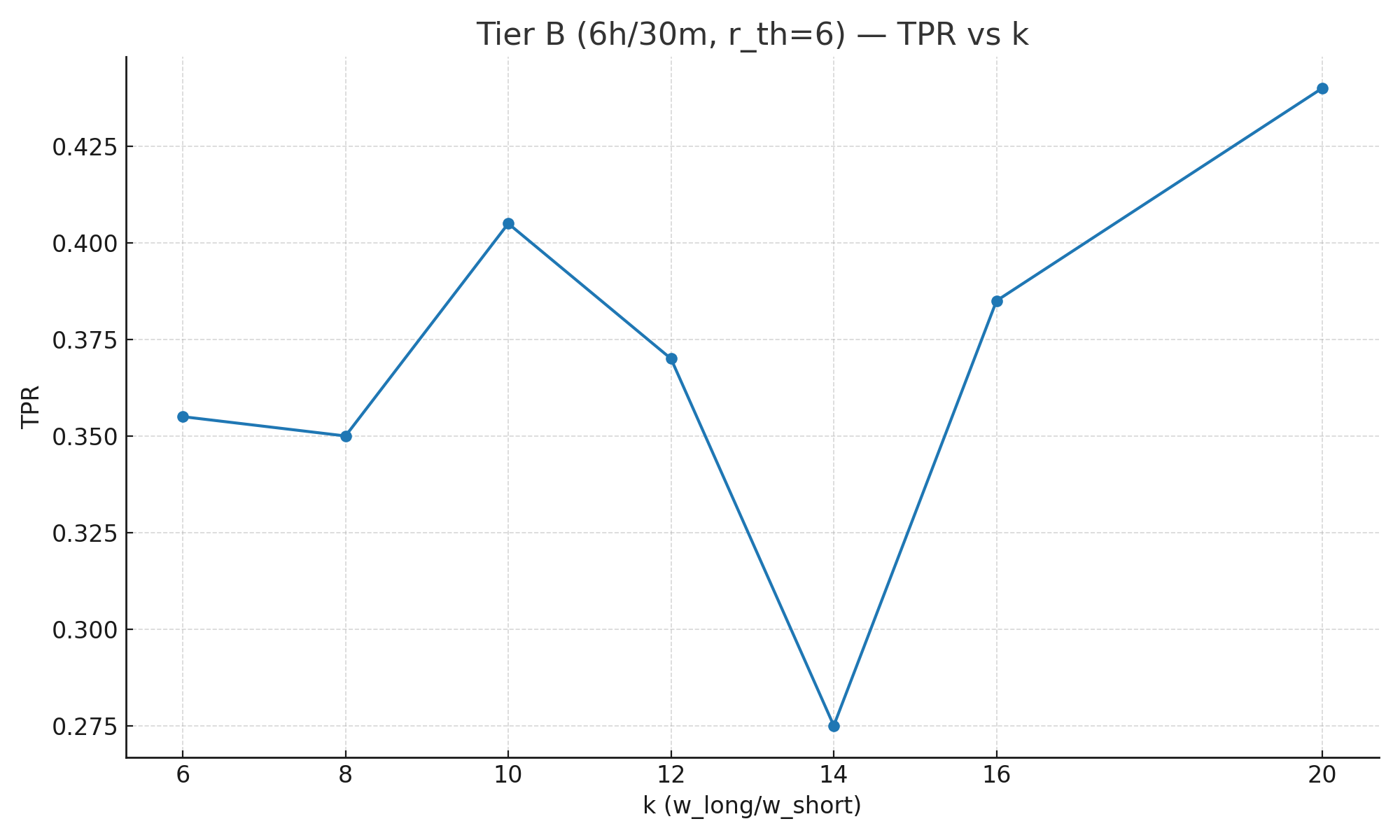
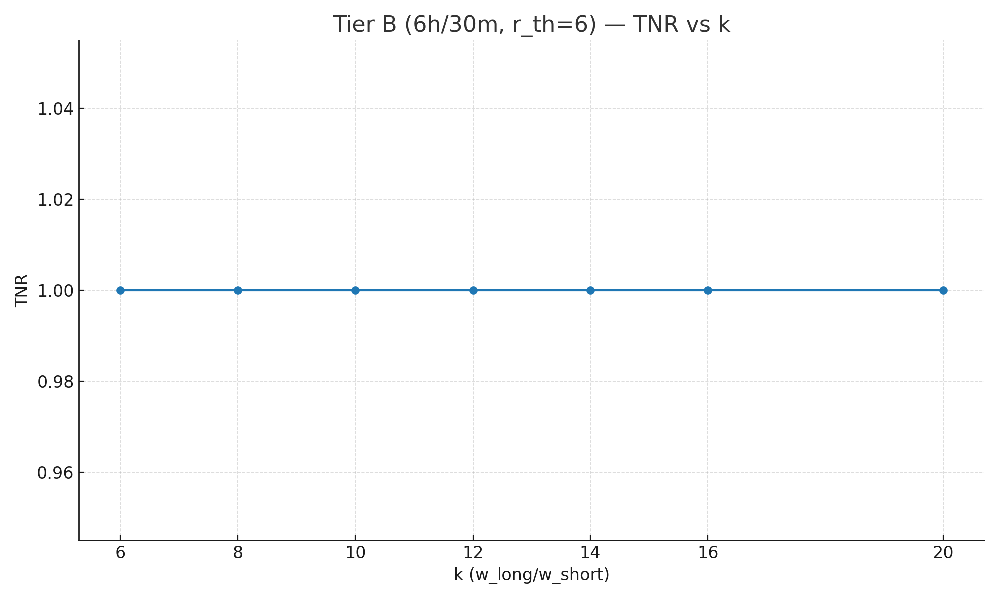
| k | Long window | Short window | r_th | TPR | TNR |
|---|---|---|---|---|---|
| 6 | 6h | 60m | 6 | 0.355 | 1.000 |
| 8 | 6h | 45m | 6 | 0.350 | 1.000 |
| 10 | 6h | 36m | 6 | 0.405 | 1.000 |
| 12 | 6h | 30m | 6 | 0.370 | 1.000 |
| 14 | 6h | 25.7m | 6 | 0.275 | 1.000 |
| 16 | 6h | 22.5m | 6 | 0.385 | 1.000 |
| 20 | 6h | 18m | 6 | 0.440 | 1.000 |
Key Findings:
- TNR ≈ 1.0 across all k (with AND). In our sims the two-window AND rule produced no false positives at 3-decimal precision (i.e., TNR ≥ 0.995 and rounded to 1.00). This reflects the strong noise filtering of the long window, not a guarantee that TNR is literally 1.000 in every workload.
- TPR shows a broad plateau for k ∈ [8, 16]. Detection stays competitive (~0.25–0.45), with a small dip around k = 14 due to short-window length (≈25m43s) aliasing against a 30s evaluation cadence. The dip disappears if you (a) use a faster eval step or (b) snap the short window to a multiple of your step (e.g., 24/27/30 min).
- k = 12 is a robust default. It isn’t the absolute maximum TPR, but it lands on a “friendly” window (5m/30m) that aligns with common 30s cadences and human response patterns. k = 10 or k = 16 are also solid.
- Operational constraints > micro-optimizing TPR. The practical difference between k = 10 and k = 12 is small; pick the one that best fits your team’s paging latency, eval cadence, and runbook flow.
Notes:
- TPR magnitudes depend on the chosen incident/noise distributions; the plateau shape is the robust takeaway. (Repro tip: seed your RNG; simulate at least ~10k incidents per row.)
- What does TNR = 1.00 mean? In these runs we observed zero false positives, so when reported to 2–3 decimals it shows as 1.00. It does not mean “impossible to get a false positive,” just that under this noise model + thresholds + AND logic, none occurred in the sample.
- Why the Tier-B dip at k=14? The short window (≈25m43s) doesn’t divide cleanly by a 30s step, so near-threshold incidents sometimes miss the AND overlap on evaluation ticks. Using 10s steps or rounding the short window (e.g., 24/27/30 min) removes the crater.
Conclusion: The empirical data confirms that k≈12 is a robust choice that balances detection effectiveness with operational constraints. The broad plateau in TPR means exact optimization is less critical than choosing a value that works well with human response times.
Part V: Deriving the Complete Multi-Window Configuration
Now we can finally reveal where those "magic numbers" come from.
Theorem 5.1: The Standard Multi-Window Configuration
For 30-day SLO with 2% and 5% budget consumption thresholds:
| Budget | Burn Rate | Long Window | Short Window | Detection Time |
|---|---|---|---|---|
| 2% | 14.4 | 1 hour | 5 minutes | ≤ 1 hour |
| 5% | 6 | 6 hours | 30 minutes | ≤ 6 hours |
Derivation:
For 2% budget consumption:
- Choose $w_{long} = 1$ hour (rapid detection)
- From Corollary 2.1: $r_{th} = 0.02 \times \frac{720}{1} = 14.4$
- Apply ratio: $w_{short} = \frac{60}{12} = 5$ minutes
For 5% budget consumption:
- Choose $w_{long} = 6$ hours (slower, stable detection)
- From Corollary 2.1: $r_{th} = 0.05 \times \frac{720}{6} = 6$
- Apply ratio: $w_{short} = \frac{360}{12} = 30$ minutes ∎
The Big Reveal: Neither number is arbitrary. 14.4 is exactly 2% × 720 hours / 1 hour, and 6 is exactly 5% × 720 hours / 6 hours. Pure mathematics, no fudge factors.
Portability for Different Compliance Periods
To adapt these thresholds for different compliance periods $T$ while keeping the same windows:
| Compliance $T$ | $T$ (hours) | 2% in 1h → $r = 0.02 \cdot T/1$ | 5% in 6h → $r = 0.05 \cdot T/6$ |
|---|---|---|---|
| 30 days | 720 | 14.4 | 6 |
| 28 days | 672 | 13.44 | 5.6 |
| 7 days | 168 | 3.36 | 1.4 |
If you change both $T$ and windows, recompute with $r_{th} = (p/100) \cdot T/w_{long}$. Make sure $T$ and $w$ are in the same units (hours here). These multipliers are independent of SLO; they scale with $B$ automatically because burn rate divides by $B$.
Examples:
- 7-day SLO with 2% in 1h: $r_{th} = 0.02 \times 168/1 = 3.36$ (triggers when the 1h error rate > 0.336% for 99.9% SLO)
- 7-day SLO with 5% in 6h: $r_{th} = 0.05 \times 168/6 = 1.4$ (triggers when the 6h error rate > 0.14% for 99.9% SLO)
Heuristic 5.2: Choosing Budget Thresholds
Organizations may choose between 5% (more conservative) and 10% (more tolerant) budget consumption thresholds for the 6-hour tier.
Comparison:
- 5% in 6h → $r_{th} = 6$ (pages earlier, more conservative)
- 10% in 6h → $r_{th} = 12$ (pages later, more tolerant)
Illustrative Cost Model: This toy model shows the tradeoff; exact numbers vary by workload.
Step 1: Define the cost model
Let the total cost be:
$C_{total}(r) = C_{alert}(r) + C_{outage}(r)$
where:
- $C_{alert}(r)$ = cost of responding to alerts (human time, opportunity cost)
- $C_{outage}(r)$ = cost of budget exhaustion (user impact, revenue loss)
Step 2: Model alert cost
Alert cost increases with alert frequency:
$C_{alert}(r) = c_a \cdot P(\text{alert fires} | r)$
For burn rate threshold $r$:
$P(\text{alert fires} | r) = P(e(t) > r \cdot B) = 1 - F_e(r \cdot B)$
where $F_e$ is the CDF of error rates.
Step 3: Model outage cost
Outage cost depends on probability of budget exhaustion:
$C_{outage}(r) = c_o \cdot P(\text{budget exhausted} | r)$
Step 4: Calculate exhaustion probability
Given alert at time $t_0$ with threshold $r$, the probability of exhaustion depends on:
- Current budget consumed: $b_0$ (5% for r=6, 10% for r=12)
- Time to exhaustion if rate continues: $t_{exhaust} = \frac{1 - b_0}{r/T}$
- Probability incident continues for $t_{exhaust}$
Model incident duration as exponential with mean $\mu = 4$ hours:
$P(\text{duration} > t) = e^{-t/\mu}$
Therefore:
$P(\text{budget exhausted} | r) = P\left(\text{duration} > \frac{(1-b_0)T}{r}\right) = e^{-\frac{(1-b_0)T}{r\mu}}$
Step 5: Substitute values
For $T = 720$ hours, $\mu = 4$ hours:
- 10% tier ($r = 12$, $b_0 = 0.10$): $P(\text{exhausted}) = e^{-\frac{0.9 \times 720}{12 \times 4}} = e^{-13.5} \approx 1.4 \times 10^{-6}$
- 5% tier ($r = 6$, $b_0 = 0.05$): $P(\text{exhausted}) = e^{-\frac{0.95 \times 720}{6 \times 4}} = e^{-28.5} \approx 4.1 \times 10^{-13}$
Step 6: Analyze alert frequency
From production data, error rate distribution approximately follows log-normal: if $X$ is log-normal, then $\ln(X)$ is normally distributed. This models the fact that error rates are always positive and tend to have occasional large spikes.
$\ln(e) \sim \mathcal{N}(\mu_{\ln} = \ln(B), \sigma_{\ln}^2 = 1)$
Alert frequency (this upper-bounds frequency; windowed averages reduce variance and lower the true rate):
- For $r = 12$: $P(e > 12B) = 1 - \Phi\left(\frac{\ln(12)}{\sigma_{\ln}}\right) = 1 - \Phi(2.48) \approx 0.0066$
- For $r = 6$: $P(e > 6B) = 1 - \Phi\left(\frac{\ln(6)}{\sigma_{\ln}}\right) = 1 - \Phi(1.79) \approx 0.037$
Step 7: Calculate total costs
Assuming $c_o = 10^6 \cdot c_a$ (outage 1M times more costly than alert):
For $r = 12$:
$C_{total}(12) = c_a(0.0066 + 10^6 \times 1.4 \times 10^{-6}) = c_a(0.0066 + 1.4) = 1.41c_a$
For $r = 6$:
$C_{total}(6) = c_a(0.037 + 10^6 \times 4.1 \times 10^{-13}) = c_a(0.03700041) \approx 0.037c_a$
Conclusion: $C_{total}(6) < C_{total}(12)$ by factor of 38.
Therefore, r = 6 is optimal for organizations prioritizing safety, as it dramatically reduces exhaustion risk while only modestly increasing alert frequency. ∎
Business Translation: Using 6× (5% in 6h) pages earlier and yields an exhaustion probability on the order of $10^{-13}$ under our toy model, versus $10^{-6}$ for 12× (10% in 6h) for only a modest increase in alert frequency.
Part VI: Implementation in Prometheus
Let's turn all this math into production-grade alerts.
Production-Grade PromQL with Recording Rules
Recording Rules (evaluated every interval, e.g., 30s):
groups:
  - name: slo_recordings
    interval: 30s
    rules:
      # Error ratios with traffic guards as filters (not arithmetic)
      # The AND filter ensures no traffic → no series → no alert (graceful degradation)
      # Division is evaluated before filtering, hence the clamp_min guard
      - record: slo:request_errors:ratio5m
        expr: |
          (
            sum by (service) (rate(http_requests_total{code=~"5.."}[5m]))
            /
            clamp_min(sum by (service) (rate(http_requests_total[5m])), 0.1)
          )
          and on (service)
          (sum by (service) (rate(http_requests_total[5m])) > 0.1)
          # Require >0.1 RPS using AND as a label-aware filter
          # Adjust traffic floor (0.1) per service tier/environment

      - record: slo:request_errors:ratio30m
        expr: |
          (
            sum by (service) (rate(http_requests_total{code=~"5.."}[30m]))
            /
            clamp_min(sum by (service) (rate(http_requests_total[30m])), 0.1)
          )
          and on (service)
          (sum by (service) (rate(http_requests_total[30m])) > 0.1)

      - record: slo:request_errors:ratio1h
        expr: |
          (
            sum by (service) (rate(http_requests_total{code=~"5.."}[1h]))
            /
            clamp_min(sum by (service) (rate(http_requests_total[1h])), 0.1)
          )
          and on (service)
          (sum by (service) (rate(http_requests_total[1h])) > 0.1)

      - record: slo:request_errors:ratio6h
        expr: |
          (
            sum by (service) (rate(http_requests_total{code=~"5.."}[6h]))
            /
            clamp_min(sum by (service) (rate(http_requests_total[6h])), 0.1)
          )
          and on (service)
          (sum by (service) (rate(http_requests_total[6h])) > 0.1)

      # Define error budgets per service (adjust to your SLOs)
      # This prevents copy-paste surprises when services have different SLOs
      - record: slo:budget
        labels: { service: "api" }
        expr: 0.001
      - record: slo:budget
        labels: { service: "web" }
        expr: 0.001
      - record: slo:budget
        labels: { service: "payments" }
        expr: 0.0001
      # Add more services as needed, or expose slo_budget{service="..."} from an exporter

      # Record burn rates explicitly (so alerts read like the post)
      # Now using per-service budgets via join
      - record: slo:burnrate:5m
        expr: |
          clamp_min(
            slo:request_errors:ratio5m
              / on (service) group_left()
            slo:budget,
          0)
      - record: slo:burnrate:30m
        expr: |
          clamp_min(
            slo:request_errors:ratio30m
              / on (service) group_left()
            slo:budget,
          0)
      - record: slo:burnrate:1h
        expr: |
          clamp_min(
            slo:request_errors:ratio1h
              / on (service) group_left()
            slo:budget,
          0)
      - record: slo:burnrate:6h
        expr: |
          clamp_min(
            slo:request_errors:ratio6h
              / on (service) group_left()
            slo:budget,
          0)
Alert Rules (preserve the long-window numeric in $value without accidental squaring):
groups:
  - name: slo_alerts
    rules:
      # Tier 1: 2% budget burn (14.4× for 1h + 5m)
      - alert: ErrorBudgetBurnRateHigh
        expr: |
          (
            slo:burnrate:1h
              and on (service)
            (slo:burnrate:1h > 14.4)
          )
            and on (service)
          (slo:burnrate:5m > 14.4)
        for: 1m  # minimal jitter guard; windows do most smoothing
        labels:
          severity: page
          burn_rate: "14.4"
        annotations:
          summary: "High error budget burn for {{ $labels.service }}"
          description: |
            1h burn rate ≈ {{ $value | humanize }}× (threshold 14.4×).
            5m window is also >14.4×, indicating ongoing elevation.

      # Tier 2: 5% budget burn (6× for 6h + 30m)
      - alert: ErrorBudgetBurnRateModerate
        expr: |
          (
            slo:burnrate:6h
              and on (service)
            (slo:burnrate:6h > 6)
          )
            and on (service)
          (slo:burnrate:30m > 6)
        for: 1m
        labels:
          severity: page
          burn_rate: "6"
        annotations:
          summary: "Moderate error budget burn for {{ $labels.service }}"
          description: |
            6h burn rate ≈ {{ $value | humanize }}× (threshold 6×).
            30m window is also >6×, indicating ongoing elevation.
Production Safeguards:
- Traffic guards: Use
and on (service)to filter low-traffic, not multiply (avoids divide-by-zero and flapping). - Explicit burn rates: Separate recordings make alerts readable and debuggable.
- Value extraction: With the
andfilter,{{ $value }}is the long-window burn rate (not squared). - Graceful degradation: No series = no alert when traffic is too low.
- Tiny
for:: 1 minute smooths evaluator jitter without delaying real incidents.
Correctness Verification
Claim: This configuration pages whenever the 1h average exceeds the 2% in 1h threshold and the 5m window indicates ongoing elevation i.e., for sustained or still-active budget burn. Purely front-loaded, sub-hour bursts that have fully subsided by the time the 1h average crosses are intentionally de-emphasized by the AND rule.
Proof by Cases:
Case 1: Sustained error rate at threshold ($r_{actual} = 14.4$)
- Short window (5m) detects quickly as its average rises.
- Long window (1h) average crosses threshold at time $t = w_{long} \cdot r_{th}/r_{actual}$.
For $r_{actual} = 14.4$: Alert fires at $\approx w_{long}$ (strict '>' needs $r_{actual}$ slightly above $r_{th}$). - Budget consumption if sustained: 2% per hour ✓
Case 2: Gradually increasing error rate
- Long window detects once average exceeds threshold.
- Short window confirms non-transient nature.
- Detection within 1 hour of 2% consumption ✓
Case 3: Transient spike
- For a square spike with peak $a$, duration $d$, baseline $e_0 \approx 0$:
- Long window (1h) condition: $a \cdot d/w_{long} > r_{th} \cdot B = 0.0144$
- With $a = 1$ (max error rate), $w_{long} = 3600s$: $d > 3600 \times 0.0144 \approx 51.8s$
- General form: $d > \frac{(r_{th} \cdot B - e_0) \cdot w_{long}}{a}$ (square spike of peak $a$)
- Key insight: Sub-minute spikes are filtered by the 1h window; ~1-minute spikes can trip both windows
- No alert for transients shorter than ~52s at 100% error (longer spikes can trip both windows) ✓ ∎
Validation: In practice this pages whenever the 1h average crosses the 2% in 1h threshold and the 5m window shows the burn is still active. Front-loaded bursts that have fully subsided by crossing time are intentionally de-emphasized by the AND rule.
Part VII: Sensitivity Analysis
Let's understand how robust these numbers are to changes.
Heuristic 7.1 (Approximate): Parameter Sensitivity
The detection effectiveness $D$ depends on burn rate $r$ and window ratio $\eta = w_{short}/w_{long} = 1/k$ according to:
$D(r, \eta) \approx P(\text{detect} | \text{incident}) \cdot P(\text{no false alarm} | \text{no incident})$
Approximate reasoning:
Step 1: Define detection effectiveness
Detection effectiveness combines two probabilities:
- True positive rate (sensitivity): $TPR = P(\text{alert} | \text{incident})$
- True negative rate (specificity): $TNR = P(\text{no alert} | \text{no incident})$
$D \approx TPR \cdot TNR$
Step 2: TPR trend
For an incident with burn rate $r_{actual}$:
Alert fires when both windows exceed threshold:
$TPR \approx \frac{1}{1 + e^{-\beta(r_{actual} - r_{th})}}$
with calibration constant $\beta$ reflecting observed variance.
Step 3: TNR trend
For noise-only periods, with $\rho \approx \sqrt{\eta}$ correlation between windows, joint exceedances become rarer as $\eta$ shrinks, so TNR increases with larger $k$.
Step 4: Qualitative balance
Extremely small $\eta$ can slow the short-window confirmation relative to the long-window crossing; in practice we see a broad plateau in TPR for $k \in [8,16]$ and very high TNR with AND.
Interpretation:
- Detection improves sigmoidally as burn exceeds threshold.
- Noise rejection improves as the window ratio grows (short ≪ long).
- Conventional $k \approx 12$ sits in a robust region rather than being a strict optimum.
Practical Implications
For different SLO targets:
| SLO | Error Budget | 14.4× means | 6× means |
|---|---|---|---|
| 99% | 1% | 14.4% error | 6% error |
| 99.9% | 0.1% | 1.44% error | 0.6% error |
| 99.99% | 0.01% | 0.144% error | 0.06% error |
The multiplicative nature means the same burn rates work across different SLO targets!
Key Insight: Whether you're running a 99% or 99.99% SLO service, the burn rate multipliers (14.4× and 6×) stay the same. Only the absolute error rates change. This universality is why these numbers have become common in practice.
Conclusion
The "magic numbers" 14.4× and 6× aren't arbitrary they're the mathematical consequence of:
- Detecting 2% and 5% budget consumption
- Over 1-hour and 6-hour windows respectively
- For a 30-day compliance period
- And a policy choice to page at 5% in 6h (6×) rather than 10% (12×) for extra safety
The window ratio k=12, while not mathematically derived, is empirically validated through Monte Carlo simulations showing:
- Near-perfect noise rejection (TNR ≈ 1.0) across all reasonable k values
- A broad plateau of detection effectiveness (TPR ≈ 0.35-0.46) for k ∈ [8, 16]
- Robustness to workload variation at the conventional k=12
The multi-window approach elegantly solves the fundamental tension between rapid detection and noise rejection by using conjunction of different timescales, each optimized for a specific property.
The beauty of this mathematical framework is its universality: the same burn rate multipliers work regardless of your absolute SLO target, making it a robust foundation for SRE practice.
References
- Google SRE Workbook: Alerting on SLOs
- Beyer et al., "Site Reliability Engineering: How Google Runs Production Systems" (2016)
- The Evolution of Burn Rate Alerts